Figures 1-3: Example Hough Transform
The Hough Transform is a useful transform for detecting a variety of shapes in digital images. This paper looks at a parallel implementation of the circular Hough Transform, designed to be used for robot tracking on a distributed memory system. A description of the algorithm is given, and the results are presented and analyzed.
The MAGICC (Multiple Agent Intelligent Coordinated Control) Robotics Lab of the Electrical Engineering Department at Brigham Young University is a test bed where various types of control, decision theory, and other robotics applications can be tested using small, circular robots. The robots (the lab currently has five of them) occupy a 15' by 15' area where they are free to move around and interact with each other. For many of these applications, it is necessary for the robots to know their position on the floor, as well as the position of the other robots. However, the current robot design does not include the sensors needed to determine this information, so each robot must depend on outside sources to obtain it.
The current solution to the problem uses a camera mounted in the ceiling above the test bed to track the robots. This camera is connected to a computer, which uses a simple program to find the robot positions and orientations from the images provide by the camera. To allow the camera to easily spot the robots, each one has a bright-colored disc placed on top of it. To determine its orientation, a smaller, contrasting disc is placed above that at the front edge of the robot. Once the position and orientation of the robots are extracted from the image, the information is transmitted via an RF link to each robot.
In order to provide suitable frame rates, the current tracking program uses a simple center of mass technique that is somewhat sensitive to noise and not always accurate. With the introduction of a robotic arm, which is sometimes is attached to the robot and obscures part of the colored disc, the center of mass technique is even more inaccurate. More robust image processing techniques, such as the Hough Transform (HT), are much less susceptible to noise and partial obstruction of the object. However, these techniques are much more computation-intensive and can not generally provide the information in a timely manner.
By devising an algorithm to compute the HT in parallel on several machines, I hoped to be able to process the images fast to provide position information to the robots at a suitable frame rate (for msot applications, this is several frames per second). The purpose of this project was to implement a parallel version of the circular HT, and to examine the speedups it was able to obtain. The program was written using MPI.
Several studies have been done on parallel implementations of the Hough transform. A good number have been conducted on SIMD parallel machines (1, 2, 3, 4), special purpose hardware (5), and shared memory systems (6). This study is somewhat unique in that it is a simple parallel implementation of the circular HT, designed using an all-purpose parallel language (MPI), and designed to run on general purpose processors using distributed memory. All of the image filters and transforms used are very simple - no specialized methods were used. While the goal of this project is very practical (to achieve faster frame rates in robot tracking), the results may prove useful to those interested in parallelizing similar algorithms on standard desktop PCs.
The HT (7) has been shown to be very efficient for the detection of shapes in images. While it can be used to detect arbitrary shapes and lines, one of the simpler versions is designed to detect circles of a given radius. This is accomplished by taking a binary image (usually generated from the source image by passing it through an edge detection filter), and, for each point, accumulating in a separate array every point which is exactly one radius distance away. This array can then be searched for peaks, which will correspond to the center of the circle(s).
This is demonstrated in figures 1-2 below. Figure 1 shows the original image, which contains four circles of different sizes. Figure 2 is an edge detected version of the first image, and is used to compute the HT. The HT is computed using a radius equal to that of the rightmost circle, and the resulting accumulator array in shown in the figure 3. Note that the peak of the accumulator array corresponds to the center of the rightmost circle.
Figures 1-3: Example Hough Transform
I divided the process of processing an image from the camera into several distinct stages, each of which will be explained in detail below. The computational and communication needs of each stage are discussed, along with the various problems that were encountered.
The stages of the algorithm are:
Input Image to Stage: 520 x 480 Color Image
To keep the image distribution simple and straight forward, row distribution is used. Each processor is given an equal number of rows to process from the image, and has at most two neighbors: one above and one below. Having only two neighbors reduces some of the communication needed in later stages of the algorithm (see sections on edge detection and the Hough Transform), which is why it was chosen instead of block distribution.
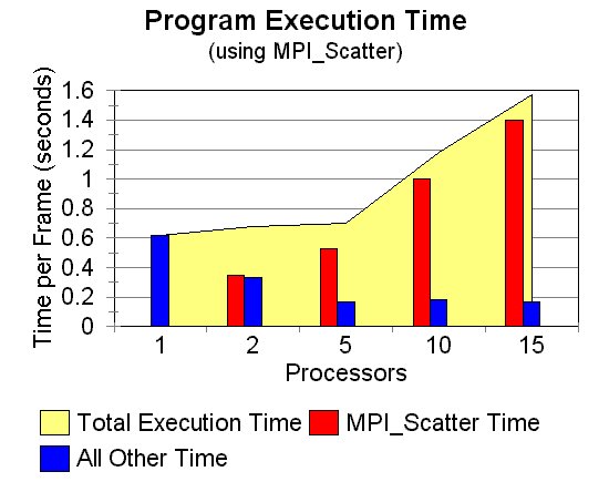
At first, MPI_Scatter was used to distribute the image. However, the time needed to distribute the image to all of the processors proved to be much greater than the computation time of the algorithm. So, as noted in the performance section, no speedups were obtained when MPI_Scatter was used.
Rather than abandon the project and call it a failure, an assumption was made that all of the processors could have simultaneous access to the source image. This could easily be accomplished by a multi-processor machine using shared memory, or possibly with a network where all of the machines could have simultaneous access to the camera. If a shared memory system is used, many aspects of the problem change and a new algorithm is needed altogether. Since particular implementation was designed to use distributed memory, the shared camera system is assumed. If this is the case, then each of the processors simply reads out their corresponding segment of the image into their own local buffer. In anticipation of the next stage of the algorithm, each processor will also read one additional row from directly above and below its segment from the image.
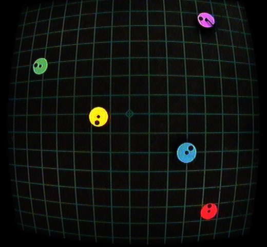
Figure 4 - A typical image received from the camera
Input Image to Stage: 520 x (480/nproc) Color Image (where nproc is the total number of processors)
The images provided by the camera, as seen in the above section, are 520x480 color images. The color can be used to distinguish between the individual robots once they are located. However, the color information is not useful when computing the HT, and only complicates matters by providing three times the needed amount of data. To remove this unneeded information, this stage reduces the image to a gray scale image. This involves averaging the red, green, and blue contents of each pixel and collapsing them into a single value.
Another useful transformation which is performed on the image at this time is a low pass filter. This helps smooth out the image, giving better results in the edge detection stage. In order to perform this convolution on the top and bottom boundaries of the image segment, the adjacent rows of the neighboring processors are needed. As mention in the previous section (see Image Distribution, these rows are simply read in from the original image so that no communication is required in this stage.
To reduce the computation time for this stage, the gray scale reduction and the low pass filter are collapsed into a single computation (several additions followed by a division). Also, for any pixels with an intensity below a certain threshold this computation is skipped altogether and the corresponding pixel value is assigned a black value (the majority of the image is black, so this avoids a lot of unnecessary computation).


Figure 5 - Low Pass/Gray Scale Reduction Filter, distributed across five processors
Input Image to Stage: 520 x (480/nproc) Gray Scale Image
Before performing the HT, it is necessary to run the image through an edge detection filter. For this implementation, a Sobel 3x3 filter is used (8). As the edge detection filter is performed, the image is also reduced to a binary image (all edges above a certain threshold are kept, while all other are lost). As with the low pass filter, the adjacent rows of the neighboring processors are needed to perform a complete filter. To provide this information, each processor sends its top and bottom rows to its upper and lower neighbors, respectively. This is done using MPI_Send, and occurs before the filter is performed.
Another problem that is addressed in this stage is the distortion of the image. As can been seen in figure 4, the image provided by the camera is distorted by the fish-eye effect. Near the edges and corners of the image, this distortion is very prominent. Unfortunately, the circular HT assumes a somewhat perfect circle in order to work correctly. Also, the distortion causes the size of the robots to vary throughout the image, making it impossible to search for a uniform radius with the HT.
To correct this problem (which is also an issue when trying to determine the exact location of each robot on the floor), a lookup table was developed [NOTE: the lookup table was developed prior to and separate from this project]. This lookup table simply maps a pixel from the current image to its corresponding position in a new, distortion-free image. The resulting image is slightly larger than the original image at 570 x 570 (leaving each processor with a 570 x (570/nproc) segment of the image). A problem that occurs when using this table is that pixels near the boundary with another processor will likely migrate to that processors space. This can be seen in figure 6 below.
To handle this migration, each processor keeps a buffer of the pixels that have migrated to its neighbors. When the edge detection filter is complete, each processor sends this buffer to its neighbors. To avoid sending the entire buffer (which could contain only a small area of actual data), the buffer is reduced in size to encapsulate the smallest possible area containing relevant data. Each processor then tells each neighbor how big the buffer is that it is going to send, where the buffer belongs in the image, and then sends buffer itself. All of these communications are done using MPI_Send. While some of the buffer sent may not contain useful information, I chose to send a block size buffer instead of each individual migrating pixel to avoid the latency involved with multiple calls to MPI_Send.
While it is possible that a pixel may migrate past a neighboring processor into the next processor (especially if nproc is large, making the data space of the processor very narrow), the frequency at which that occurs for this particular application does not justify the overhead of checking to see if it has occurred. However, it could be handled in a similar manner.
Also, as previously mentioned (see Image Distribution), the use of row distribution limits the amount of neighbors that each processor can have to two. If block distribution were used, a processor could have up to four neighbors. This could double the number of communications needed to handle the migrating pixels, which would most likely cause a decrease in performance (since, as noted in the results, the communication time required is already somewhat large).


Figure 6 - Results of Edge Detection/Fish-Eye Correction Filter distribute across five processors. The area boxed in yellow denotes pixels which migrated from one processor to another due to the fish-eye correction. Compare with figure 5.
Input Image to Stage: 570 x (570/nproc) Binary Image
Now that the image has been edge detected, the HT can be performed as outlined previously. For each pixel in the input image, a series of computations using sines and cosines are used to determine the points that are exactly one radius away from that pixel. To speed these computations, a lookup table is used to determine the values of the sines and cosines. This reduces the computation for each pixel to a series of multiplies to compute the accumulator array.
There is some communication that must be performed, however, in order to complete the transform. It is possible that the computed accumulator array will not stay entirely within the data segment of the processor - part of the accumulator array may belong to neighboring processors. When this happens, it is handled in the same way that migrating pixels are handled in fish-eye correction.
For this application, the HT is performed twice on each image. The first HT produces the accumulator array for the robot positions, so the radius of the transform is set to match that of the robot. The second HT uses a radius equal to that of the orientation mark on the robot. The resulting accumulator array can then be used to find the orientation marks on the robots to determine which direction they are facing.


Figure 7 - Resulting accumulator array from the Hough Transform, distributed across five processors. The areas outlined in red denote pixels which migrated from one processor to another during the computation. [Note: The image has been inverted so that the accumulated points are easier to see.]
Input Image to Stage: 570 x (570/nproc) Accumulator Array
Once the HT has been performed, the final step is to search the resulting accumulator arrays to find the center coordinates of the circles. The basic search consists of each processor searching its part of the array for peaks, and then all of the processors communicating to determine which one has the largest peak. However, locating the center of the robots and locating the center of their orientation marks is not accomplished in exactly the same way. Each process is explained below.
The first peaks that are found are those in the accumulator array containing the robot positions. For n robots, each processor makes n passes through its segment of the accumulator array and remembers the highest point found in each pass, placing it in a potential peak list. It then goes back through the accumulator array and wipes out all of the data within a radius distance of that point (actually, for simplicity it wipes out a 2r x 2r block centered around the peak, where r is the radius of the robot). The reason for doing this is so that the next peak found will be guaranteed not to be located on the same robot as the last peak. If no peak is found in the accumulator array (either because it was empty to start with or all of the useful data has been wiped out in previous iterations), the search is stopped.
Once each processor has found up to n peaks in its data segment, all of the processors communicate to determine where the n global maxima are in the accumulator array. To accomplish this, n calls to MPI_Allreduce are used. Each processor encodes an integer with three values: the peak value, the x coordinate of the peak, and the y coordinate of the peak. This is done using the following formula:
value = peak * 1000000 + xcoord * 1000 + ycoord
MPI_Allreduce is then called with this value. (If the processor has run out of peaks to submit, it simply submits a value of 0). The result is that each processor will end up with an integer corresponding to the highest peak value, and can extract the x and y coordinates from it. If the x and y coordinates match those of its own peak value which was submitted, it removes that value from its potential peak list and submits its next highest peak to the next call to MPI_Allreduce.
Another situation that can occur is when two processors submit a peak value that is located on the same robot (referred to here as conflicting peaks). While each individual processor is guaranteed to not have conflicting peaks, there is no guarantee that this will not happen with neighboring processors (and it is likely to happen if the center of the robot is located near a boundary between the two processors). To prevent this, after each call to MPI_Allreduce, each processor (except for the processor who submitted the maximum peak for that iteration) compares the coordinates of all of the peaks in its potential peak list to that of the peak that was just accepted. If any of the peaks conflict, they are removed from the potential peak list of that processor. In this manner, after n calls to MPI_Allreduce, each processor has a list of the coordinates of each of the robots in the image.
The search for finding orientation peaks is somewhat simplified from that of finding the robot positions. Since there is only one orientation peak per robot, and each processor now knows the location of the robots, the search can be limited. Each processor makes n passes through its accumulator array for the orientation positions. For each iteration i, the processor searches the space in the accumulator array that it within one radius distance (again, it actually searches a block of size 2r x 2r) from the center position of the ith robot. If no part of the 2rx2r search window lies within that processor's segment of the accumulator array, it simply skips ahead to the next iteration. The peak that is found (if any), is stored as a potential peak for the ith robot.
Once the peaks are located, the processors communicate to determine the orientation peak positions. This is done by using MPI_Allreduce in much the same way that the robot peaks are detected. The notable difference is that each peak in the potential peak list now corresponds to a specific robot (If the processor does not have a candidate for the orientation peak for a specific robot, it simply submits a zero for that iteration). In this manner, the first call to MPI_Allreduce determines the location of the orientation mark of the first robot (as found with the previous peak detection), the second call determines the second, etc. After n calls to MPI_Allreduce, each processor knows the location of the orientation marks of each robot.
As mentioned when discussing image distribution, absolutely no speedups were obtained when MPI_Scatter was used to distribute the image to the processors. Below in graph 1, we see the average timing results for 10 frames processed on 1, 2, 5, 10, and 15 processors using MPI_Scatter. As the number of processors increases, the total percentage of the time taken by the call to MPI_Scatter increases as well. If the computation time per frame was much greater than that of the call to MPI_Scatter, speedups could be achieved. However, since the computation time per frame is small (and has to be, in order to achieve the high frame rates necessary for the robotics applications), distributing the image with MPI_Scatter is not acceptable for this implementation.
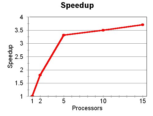
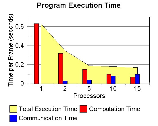
When the simplifying assumption is made that all processors can access the source image simultaneously, we can see some limited speedup results (see graph 3). Good speedups are obtained for runs on 2 and 5 processors, but after that it levels off. It is interesting to note in graph 2 and table 1 that while the computation time decreases for 10 and 15 processor slightly, the communication time offsets the decrease.
| Processors | Computation Time |
Communication Time* |
Total Time | Speedup | Frames/Second |
|---|---|---|---|---|---|
| 1 | 0.63 | 0.0 | 0.63 | 1.0 | 1.59 |
| 2 | 0.32 | 0.03 | 0.35 | 1.8 | 2.86 |
| 5 | 0.14 | 0.05 | 0.19 | 3.32 | 5.26 |
| 10 | 0.10 | 0.08 | 0.18 | 3.5 | 5.56 |
| 15 | 0.07 | 0.10 | 0.17 | 3.71 | 5.88 |
Why does the performance level off after only five processors? It is most likely due to a combination of factors:
Because the majority of the image is black, there is not a lot of data to process in the image. After dividing up the image into so many segments, there is so little data on each processor that any further division of the data does not decrease the computation time significantly. This is also due to the next problem...
This algorithm currently uses no load balancing to distribute the data. If all of the robots are concentrated in the same area on the floor, then several processors could be left with nothing to do. This limits the reduction of the overall computation time.
As seen in (graph), the time spent in communication grows with the number of processors. As more processors are added to help increase the performance, the communication time rises to counter some (or all) or the benefit gained.
By the nature of the HT, this is a communication intensive problem. Ignoring the fish-eye correction, which is specific to this application, there is still the merging of accumulator arrays between processors and global peak detection which require communication. For best results in parallel processing, such communication is undesirable.
There is a lot that could be done to improve on this implementation of the circular Hough Transform. Some of these areas are:
There might be faster and better ways to compute some of the image filters that are implemented in this program. Being a novice at image processing, I used very standard and well known methods for all of the filters.
By distributing the load more carefully across the processors, higher speedups might be obtained. However, this could possibly cause communication time to increase slightly as more pixels are migrating between processors.
The current method of peak detection could probably be improved upon. Perhaps a scheme where each processor sent its potential peak list all at once to the root node, where the best peaks were then extracted locally would provide better performance. However, the global communication in this stage can not be eliminated entirely.
Based on the performance of this program, it appears that a parallel implementation of the Hough Transform on general purpose processors using distributed memory is a bad idea. If all of the processors can access the image simultaneously, it is possible to achieve a limited speedup on a small amount of processors. However, the feasibility of accessing an image in this manner has not been investigated.
The reasons for the poor performance, as mentioned above, suggest that the HT is best suited for shared memory systems. In a shared memory system, almost all of the communication issues disappear. The image can be accessed by all processors, and each processor can update any part of the accumulator array without communicating with the other processors. This leaves only the problem of how to divide up peak detection, which can be handled in a number of different ways (since each processor has access to the entire accumulator array).
This study suggests that any problem with limited computational requirements must be dealt with carefully when being split into a parallel algorithm. If there is a fair amount of communication required within the algorithm, the overhead of implementing it in parallel could very well offset the computational savings. Such problems are best left to shared memory systems if they are to parallelized in real time environments.