Abstract
The floorplan optimization problem is an important algorithm used
extensively by the semiconductor industry. The huge amount of time required
to find an optimal answer using a single processor makes the problem a
prime candidate for parallel processing. The floorplan optimization problem
is reduced to the bin packing problem and serial and parallel implementations
are developed. Comparison of the execution times of the parallel implementation
to the serial implementation indicates that superlinear speedups are attainable
for most data sets.
Introduction
The cost of producing a chip is often dominated by the total area of the silicon wafer required. Optimal utilization of silicon wafer area has two parts, shrinking the size of an individual transistor and arranging the transistors on the silicon in such a way as to minimize the area used by the entire circuit. The latter part is referred to as the floorplan optimization problem. To reduce the cost of a chip, i.e. increase profits, the industry has pumped millions of dollars into researching ways to efficiently solve the floorplan optimization problem.
The floorplan optimization problem is NP-complete which implies that an optimal solution is difficult to find in a reasonable amount of time [Mcf]. During the 1980s and early 1990s hundreds of proposals were made and programs written to obtain solutions to the problem in a reasonable amount of time. Most of the implementations were executed on a single processor and involved either an exhaustive or a heuristically guided search of a large space of possible solutions [Ban]. Even with complex heuristics, the vast majority of the implementations still required hours (sometimes days) to find an optimal solution. Programs that are used today by the semiconductor industry often sacrifice finding the optimal answer for obtaining a faster execution time [Fos].
The huge amount of time required to find an optimal
answer makes the floorplan optimization problem a prime candidate for parallel
processing. For this project, the floorplan optimization problem is reduced
to the bin packing problem (which is also NP-complete.) A serial and parallel
implementation of the solution to the bin packing problem is created. Comparing
the execution times of the parallel implementation to the serial implementation
indicates that superlinear speedups are attainable for most data sets.
Problem Description
Floorplanning is the non-overlapping placement of rectangular blocks (transistor circuits), each with a fixed area but unknown dimensions, into an area with a specified maximum width and height. Placement is limited by connectivity requirements among the blocks and by the available placement area. An optimal floorplan is one in which the total area of the blocks is a minimum (area is defined as the product of the maximum horizontal and vertical extents) and all the connectivity requirements are satisfied [Fos][Ban][She].
In the interest of time, the connectivity constraints were removed and the dimensions of each block were fixed. These modifications effectively reduce the floorplan optimization problem to the bin packing problem. While removing the connectivity constraints makes finding the solution to the bin packing problem more general than finding the solution to the floorplan optimization solution, it has been shown that since the bin packing problem is a subset of the floorplan optimization problem, any improvements made to the bin packing algorithm also improve the performance of the floorplan optimization algorithm [SSR]. Thus, it is reasonable to implement the bin packing algorithm and save adding the constraints for another project.
The bin packing problem involves packing a collection
of rectangles into an open-ended fixed width bin. The packing is orthogonal
(an edge of any packed rectangle is parallel to either the bottom or sides
of the bin), no two pieces may overlap, and the rectangles can be rotated.
An optimal solution is one in which the height of the rectangles packed
into the bin is a minimum [BCR]. For the sake of simplicity, the dimensions
of the blocks and of the bin can only take on integer values.
An Algorithm to Solve the Bin Packing Problem
A solution to the bin packing problem is found by placing
the blocks in the bin one at a time in a left most best fit (LMBF) fashion,
i.e. each piece is placed in the lowest possible location in the bin and
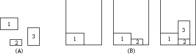
then left-justified at its vertical position. Figure 1A shows a group of
blocks and Figure 1B shows how each block is placed in the bin in LMBF
fashion. This solution is not guaranteed to be optimal (the packed bin in
Figure 1B does not have an optimal height) but if the blocks are placed into
the bin in order of decreasing width, the solution is always close to the
optimal one [BCR].
|
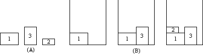
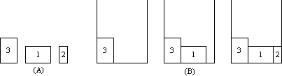
An optimal solution to the bin packing problem is
found by first organizing the group of blocks into a list. Next all the
permutations of the list are generated, taking into account that each piece
can be rotated 90 degrees. Each permutation of the original list dictates
the order in which the blocks will be placed into the bin. A bin is then
packed in LMBF fashion for each permutation. Finally, all the packed bins
are examined and the bin with the lowest height is the optimal solution.
There is commonly more than one optimal solution per set of blocks. Figures
2 and 3 show the bin packing steps for two different permutations of the
set of blocks in Figure 1A.
 |
 |
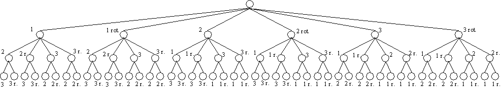
The algorithm described above can be implemented
by traversing an n-ary search tree where each node in the tree corresponds
to placing a single block in the bin using the LMBF method. The search
tree for a three block set is shown in Figure 4. Each permutation of the
block list is generated by doing a depth first traversal of the tree. Every
leaf node represents a fully packed bin. Each time a leaf node is reached,
the height of the packed bin is compared to the best height found so far,
replacing the best height if the new height is smaller. Traversing the
entire tree yields the optimal solution.
 |
The Serial Bin Packing Algorithm
My serial version of the bin packing algorithm, uses recursion to generate and traverse the search tree. The bulk of the computation done within the recursive procedure involves finding the proper location in the bin to place the next block. The location is found using an algorithm similar (but not identical) to the mixed-integer programming model [SSR]. A search of the bin is performed, looking for a free location starting at the bottom left of the bin and moving to the right. This left-to-right search is repeated on every row until a location is found. If the block to be placed is too wide to fit in the location (it overlaps with another block or with the bin boundaries), the search continues until the next available location is found. This process is repeated until the block is placed.
The block placement method explained above works but is by no means efficient. An efficient method would involve solving the city skyline problem with overhangs and enclosures. The implementation of that algorithm is quite complicated and well beyond the time constraints for this project.
Traversing the entire recursion tree using my serial algorithm is time consuming, even for small data sets. For example, a ten block set requires a search tree with 6, 126, 468, 861 nodes and takes 27 hours to traverse using an HP Visualize C180 workstation. Reducing the number of nodes is obviously a necessity.
Two heuristics are employed to prune branches of the search tree, the use of a seed and the use of a lower bound. A seed is computed by sorting the blocks by decreasing width and using the LMBF method to place them in the bin, starting with the widest block. This method does not account for block rotation but does provide a relatively good height to start with. As the tree is traversed, the height of the partially packed bin at each non-leaf node is compared against the seed. If the height exceeds the seed then the children of the node cannot produce an optimal answer and are subsequently pruned. As leaf nodes are traversed, the seed is eventually replaced with the best height found "so far" [KGGK]. The use of a seed and best height comparison reduced the execution time of the serial algorithm on a ten block data set from 27 hours to 11 hours.
A lower bound is the smallest height that can be achieved if the blocks where ground into small particles and dumped into the bin. It can easily be shown that the optimal height must be equal to or greater than the lower bound. The lower bound is found by summing the area of all the blocks, dividing the sum by the width of the bin, and rounding the resulting value up to the nearest whole integer. At each leaf node, the height of the packed bin is compared to the lower bound. If the height equals the lower bound, then an optimal answer has been found and the program quits. For the ten block data set mentioned above, using a lower bound reduced the execution time of the serial algorithm from 11 hours to 87 seconds, a speedup of 460! Utilizing a lower bound only reduces execution time for data sets where the optimal height is equal to the lower bound. But out of 34 randomly generated data sets that were used during testing, none had an optimal height that was greater than the lower bound so the use of a lower bound is justified.
Table 1 gives some sample execution times of the
serial algorithm on various random data sets.
The Parallel Bin Packing Algorithm
The bin packing algorithm described above lends itself well to parallelization. The search tree is large and can easily be dissected. Each of the tree branches can be traversed by a different processor and a managing processor can collect and analyze the results. However, this algorithm poses some interesting problems because the size and shape of the search tree are not known ahead of time. Also, the need for reducing the tree size by pruning introduces the need to periodically broadcast the best results.
I chose to implement the parallel algorithm using a root processor as a centralized job manager that controls a dynamic load balancing scheme. The root processor begins by computing a seed and a lower bound and broadcasting it to all the other processors. It then expands the search tree down to the second level (the root node is the zero'th level) and waits for work requests from the other processors.
When a processor has been initialized it requests work from the root processor and subsequently receives a node. It expands this node and traverses all its branches in a depth first manner. The processor makes use of the seed and the lower bound to prune the tree. After traversing 15,000 nodes, the processor sends its best height found so far to the root processor where it is compared to the global best height. The root processor sends the smallest of the two heights back to the processor where it replaces the local best height and traversal continues. This "check in" with the root repeats after the traversal of every 15,000 nodes. After the initial node has been completely expanded and traversed, the processor requests more work from the root and the cycle repeats. If no more work is available, it sends its final best height to the root processor and waits for further instruction from the root processor.
Once the root processor has distributed all the work,
it waits for all the other processors to finish, collects the best height
from each one, and prints the results.
Analysis of Results
The parallel bin packing algorithm was executed on
a cluster of HP workstations using 34 randomly generated data sets as input.
Table 1 displays some sample execution times of the parallel algorithm
on a few of those data sets. As expected, the execution time of the
parallel algorithm is always greater than the execution time of the serial
algorithm (with the exception of very small data sets.)
|
|
Parallel 12 Proc. |
Parallel 16 Proc. |
Parallel 20 Proc. |
Parallel 24 Proc. |
|
| 8 Blocks | 2.88 | 0.88 0.30 |
1.19 0.41 |
1.20 0.71 |
3.41 1.83 |
| 10 Blocks | 86.95 | 4.67 1.14 |
7.48 3.00 |
6.58 1.96 |
7.95 3.10 |
| 11 Blocks | 769.52 | 15.89 4.93 |
18.06 4.05 |
19.93 7.39 |
16.72 5.68 |
| 12 Blocks | Halted After 28 Hours | 9.56 2.24 |
11.49 4.05 |
11.56 4.61 |
11.58 4.33 |
| 14 Blocks | Days | 13.33 5.34 |
7.49 1.37 |
12.61 6.58 |
11.31 6.27 |
| 50 Blocks | Weeks | 834.20 27.86 |
75.40 46.43 |
61.15 34.14 |
48.36 23.85 |
The most striking observation gleaned from the test runs of the parallel algorithm is that the performance of the algorithm is heavily dependent on the size and ordering of the blocks in the data set, rather than the number of blocks in the data set. For some data sets, the optimal solution is found within the expanded trees of the first few nodes handed out by the root processor. Since the optimal height is usually equal to the lower bound, no more searching is required and the algorithm is terminated rather quickly. But for other data sets, the optimal solution is located in one of the last nodes to be distributed and may take hours to find, particularly in the cases where the optimal height does not equal the lower bound. For example, it took 8 hours using 12 processors to find an optimal solution to one particular 14 block data set while a different 14 block data set took a few seconds using the same number of processors. This search anomaly is common for many NP-complete problems [AKR].
When designing a parallel algorithm, it is preferable to find a mathematical equation to model its execution time. Among other things, this allows the designers to compute an ideal speedup and compare it to the measured speedup. Unfortunately, due to the previously mentioned search anomaly, it is nearly impossible to formulate such a model. Speedup is different for every data set.
The aforementioned search anomaly makes it difficult to determine the scalability of the algorithm. If the optimal answer for a large data set is found quickly using a fixed number of processors, adding more processors to the problem will only increase the overhead. This is especially evident from the execution times for the 14 block data set presented in Table 1. But for other data sets, adding more processors greatly improves performance. The 50 block data set in Table 1 is one such example. In general though, adding more processors increases the performance of the algorithm.
It should be mentioned that the blocks in the 50 block data set in Table 1 are small to ensure that the optimal height is equal to the lower bound. But in general, a 50 block data set is too large to be solved in a reasonable amount of time using this algorithm. I found that the optimal solution for most data sets with more than 13 blocks could not be found in less than a day. This is due largely to the inefficiency of the block placement algorithm as described in the Parallel Bin Packing Algorithm section of this paper. Since this algorithm is executed millions of times (billions for large data sets), any improvement in its execution time would increase the performance of both the serial and parallel bin packing algorithms. The parallel algorithm must be improved if it is to have practical use in the semiconductor industry. Typical floor plans have more than 1000 blocks.
Examination of the execution times in Table 1 shows that a large percentage of processor time (usually 30% to 50%) is spent doing nothing. In particular, notice the idle time for the 50 block data set. One might theorize that communication bottlenecks between the root processor and all the worker processors is the cause of this large amount of idle time. But some simple tests show that the computation time for each processor greatly exceeds the communication time. In fact, the communication time for each processor is always less than one second, regardless of which data set is being used as input (at least for all the test data sets I generated.) Almost all of the idle time occurs after there is no more work to be distributed. It turns out that most of the processors are waiting for one or two other processors to complete their assigned workload. If a processor exchanges best heights with the root processor every 15,000 traversed nodes, such delays should have been minimized but it was found that the slow processors in question were also executing heavy workloads from other users. Thus we can see that one bogged down processor can dramatically increase execution time.
One way to reduce the idle time would be to implement
a dynamic load balancing scheme based on the number of computation cycles
that a processor can dedicate to the execution of the algorithm. Another
method would be to reduce the size of the individual workloads that are
distributed by the root processor. While this would increase communication
time, slow processors would be able to finish jobs quicker.
Future Work
There is much that can be done to improve the performance of the parallel bin packing algorithm. A few suggestions are:
Conclusion
My parallel implementation of the bin packing problem
routinely outperforms the serial implementation sometimes acquiring speedups
in the thousands. However, most data sets with more than 13 blocks take
an unreasonable amount of time to solve. The inefficient placement algorithm
needs to be improved so that larger data sets can be used. The algorithm
would then have more practical uses in industrial applications. Different
dynamic load balancing schemes may also help improve performance. The parallel
implementation is very promising for future use in floorplan optimization
applications.
References
[AKR]   S. Arvindam, V. Kumar, and V. Rao, "Floorplan Optimization on Multiprocessors,"
        in Proc. 1989 Intl Conf. on Computer Design, IEEE Computer Society, 1989, pages 109-113.

[Ban]   P. Banerjee, Parallel Algorithms for VLSI Computer-Aided Design,
        Prentice Hall, New Jersey, 1994.

[BCR]   B. S. Baker, E. G. Coffman, Jr, and R. L. Rivest, "Orthogonal Packings in Two Dimensions,"
        in SIAM Journal on Computing, Vol. 9, No. 4, 1980, pages 846-855.

[CGJT]  E. G. Coffman, Jr, M. R. Garey, D. S. Johnson, and R. E. Tarjan,
        "Performance Bounds for Level-Oriented Two-Dimensional Packing Algorithms,"
        in SIAM Journal on Computing, Vol. 9, No. 4, 1980, pages 808-826.

[Fos]   I. Foster, Designing and Building Parallel Programs,
        published on the Internet at http://www-unix.mcs.anl.gov/dbpp/, Chapter 2.

[HGF]   A. Herrigel, M. Glaser, and W. Fichtner, "A Global Floorplanning Technique for VLSI Layout,"
        in Proc. 1989 Intl Conf. on Computer Design, IEEE Computer Society, 1989, pages 92-95.

[KGGK]  V. Kumar, A Grama, A. Gupta, G. Karypis,
        Introduction to Parallel Computing, Design and Analysis of Algorithms,
        Benjamin/Cummings Publishing Company, Redwood City, California, 1994, Chapter 8.

[Mcf]   M. C. McFarland, "A Fast Floor Planning Algorithm for Architectural Evaluation,"
        in Proc. 1989 Intl Conf. on Computer Design, IEEE Computer Society, 1989, pages 96-99.

[Pea]   J. Pearl, Heuristics, Intelligent Search Strategies for Computer Problem Solving,
        Addison-Wesley, Reading, Massachusetts, 1984.

[She]   N. Sherwani, Algorithms for VLSI Physical Design Automation, 2nd Edition,
        Kluwer Academic Publishers, Norwell, Massachusetts, 1995.

[SSR]   S. Sutanthavibul, E. Shragowitz, and J. B. Rosen,
        "An Analytical Approach to Floorplan Design and Optimization,"
        in IEEE Transactions on Computer-Aided Design, Vol. 10, No. 6, 1991, pages 761-769.

[WKC]   S. Wimer, I. Koren, and I. Cederbaum, "Optimal aspect ratios of building blocks in VLSI,"
        in Proc. 25th ACM/IEEE Design Automation Conf., 1988, pages 66-72.