High dimensional integrals occur frequently in many and varied fields. Often such integrals cannot be directly evaluated and some approximation technique must be used. In many cases, the Monte Carlo method provides the best means of approximation. Since it is based on random sampling, though, large numbers of samples (on the order of 108) must be obtained, which, depending on the integral, can be fairly expensive to evaluate. This paper focuses on parallelizing Monte Carlo methods for integral estimation, and includes in its analysis integrals whose intervals are bounded by functions of the variables of integration instead of just constants. Algorithms are implemented and tested, and data is collected and analyzed on a parallel system. Experiments show that the speedup obtained using parallel techniques is close to ideal.
High dimensional integrals are frequently encountered in diverse fields such as statistics,
economics, mathematics, and physics to name just a few. In these fields, the uncommon case
is that such integrals can be directly evaluated, and even then the process is difficult at
best. Most commonly, however, such integrals either cannot be directly evaluated or
have no closed-form solution, making a direct solution impossible. For one-dimensional
integrals with these problems, several numerical analysis techniques exist, such as
quadrature, that can be used to provide accurate estimates [Bur]. Unfortunately, such
techniques become increasingly complex in higher dimensions, and they give results that are
much poorer than their 1-dimensional counterparts [Shr]. The problem is compounded even
further when nonconstant intervals of integration are allowed; i.e., the intervals of
integration are functions of the variables of integration. Examples of such integrals
are (hereafter referred to as integral 1 and integral 2, respectively):
For problems of this nature, Monte Carlo methods are arguably the best technique for estimating their value. Unlike quadrature or other numerical analysis methods, the complexity of Monte Carlo methods for integral estimation is independent of the dimension of the problem. Also, their accuracy is determined primarily by the number of points to be sampled (see figure 1), so that it can be tuned by the user.
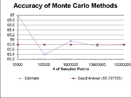 |
| Figure 1 Accuracy of Monte Carlo methods for increasing numbers of sampled points |
Fortunately, estimation is a computationally-bound problem, making it ripe for parallelization. Since each (uniformly) sampled point is generated independently of the other points, parallel algorithms can be developed that require very little inter-processor communication and give near optimal speedup results.
Using the Monte Carlo method to estimate definite integrals is a well-researched area. So also is the field of parallel Monte Carlo techniques in general. However, using parallel Monte Carlo methods to estimate high-dimensional integrals seems to be an area that has slipped through the cracks. Frequently mentioned is the fact that Monte Carlo methods are easy to parallelize for solving one- or two- dimensional integrals, especially those without a closed form solution [Har][Whi]. However, mention is not made of their applicability to higher dimensional integrals, in particular, those with nonconstant intervals of integration. This paper attempts to fill in the gap described above. Emphasis is placed specifically on the feasibility of estimating high-dimensional integrals using parallel Monte Carlo techniques.
The term "Monte Carlo Method" is a general term describing a family of techniques for solving problems by random sampling. Developed in the late 1940's, it takes its name from the casino-laden city of the same name in the country of Monaco, because roulette wheels are one of the simplest machines available for effectively generating random numbers. Some specific problems to which this technique can be applied include flow-shop scheduling, calculating quality and reliability of devices, radioactive decay, and particle transmission. For estimating definite integrals, there are two commonly used techniques. The first involves estimation of the mean of a function; the second uses a geometric approach to approximate the "area" under the curve to be integrated.
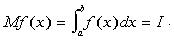
To compute the integral using mean estimation techniques, we must first find an appropriate pdf
p(x) (A pdf or probability density function is any function p(x) such that
 ). Although any pdf can be used, the closer it
is to the integrand, the more accurate the results will be. Suppose we are trying to find the
solution to
). Although any pdf can be used, the closer it
is to the integrand, the more accurate the results will be. Suppose we are trying to find the
solution to  . The mathematical expectation is given by
The geometric or area-sampling method, while not as precise, is much more intuitive and easier to extend to higher dimensions. Using this method, we estimate the area under the curve compared to the (known) area of a bounding box that encloses the curve and its associated intervals of integration.
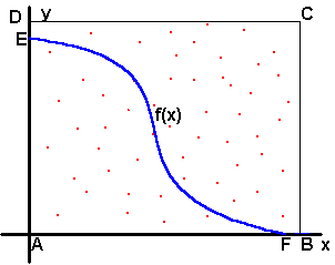 |
| Figure 2 Uniformly distributed random points fired into a box that bounds the function f(x) |
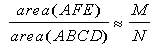
Using Figure 2 as a guide, let area(AFE) denote the true area under curve f(x) over the
interval A to F (the area we are trying to find), and let area(ABCD) denote the area of the
box ABCD, which bounds area (AFE). Generate N random points uniformly distributed throughout
the box and fire them into the bounding box. Suppose that we are able to determine that that
M of the N points fired actually fall under the curve f(x). Then, since the N random points
have a uniform distribution, we can establish the relationship
 , we can estimate the integral as
 .
.Extending the area-sampling approach to multiple dimensions is straightforward. For a one-dimensional integral, we generate and fire a 2d random point into a bounding box; for a two-dimensional integral, we generate and fire a 3d random point into a bounding cube and count all the points that fall underneath the surface of integration. Higher dimensions extend identically.
Although the mean estimation method produces more accurate estimates with fewer samples, area-sampling is much more intuitive (both the method itself and your ability to comprehend how it works in higher dimensions), and it scales to multiple dimensions much more easily. Therefore, for this paper, the area-sampling method is the technique that has been implemented.
Despite the superiority of the first method over the second, both have the property that the error decreases as the inverse square of the number of samples (see figure 3). Furthermore, this rate of decline is independent of the number of dimensions. So, although traditional one-dimensional numerical analysis techniques may have better error rates than Monte Carlo methods, the simplicity of the method and its dimension-independence properties make it ideal for high-dimensional integrals for which the traditional methods fail[Har].
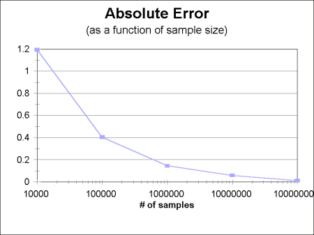 |
| Figure 3 Absolute Error of integral 1 for increasing sample sizes |
Implementing the area-sampling method to run in serial is a straightforward process even for multiple dimensions. In one dimension, we generate a 2d point (x1, x2) and ask if it falls underneath the curve and within the interval of integration (there is only one interval in this case). If it does, we "accept" it by incrementing the number of accepted points. Otherwise, we reject it and increment the number of rejected points.
In multiple dimensions, the process is the same. For a d-dimensional integral, we generate a uniformly distributed d+1 dimensional point and determine whether or not it falls under the surface of integration and within the intervals of integration. If the intervals happen to be nonconstant, we simply test the value of the point in each dimension against the integration interval for that dimension. Figure 4 contains the serial algorithm described above.
The algorithm in figure 4 assumes that the bounding box for the integral is known. Although, a bounding box is not generally included when an integral is to be solved, it can be determined easily. Since the outermost interval in an integrand must be constant (otherwise the integral cannot be completely solved), we can use the constant values to find the maximum value of the interval in the next dimension, and so forth. For example, the first integral in section 1 has the range 0..2 in its outermost interval (the x-dimension). Using these values for x, we can calculate that the y dimension (which ranges from 0 to x) can be enclosed by a bounding box with extents 0..2. In the z-dimension, which ranges from 0 to x+y, we calculate that the maximum value is 4, so that 0..4 specifies the bounding region in this dimension.
|
The heavy computational requirements (each generated point must be evaluated by potentially several functions) and minimal communication needs combined with the large number of points to be generated make this application of the Monte Carlo Method a prime candidate for parallelization, While many decomposition techniques involving exotic communication schemes can be developed, the simplest and fastest decomposition simply divides the number of points we want sampled among the available processors. This is because it is generally much faster for a processor to compute whether or not a point lies within the area of integration than it is to invoke a communication sequence along with its associated overhead. For p processors then, each processor effectively estimates the integral using N/p sampled points.
Cross-processor communication is required only at the beginning of the estimation process and at the end. Assuming that each processor has all the required information (functions, intervals, etc) (see section 6), the only initial communication that is required is to desynchronize random number generation; i.e., we must ensure that no processor is generating the same sequence of random numbers as any other processor involved in the computation.
To ensure that this desynchronization occurs, a very simple process is used. Processor 0 seeds its random number generator with a standard call (srand(time(NULL))). It then generates and sends a random number to each processor involved in the computation. Each of these processors uses the number it received to generate its own seed. Although this technique guarantees that the same sequence won't be used by more than one process and was sufficient for this project, it does have its weaknesses. Better distributed random number generators exist [Alu]. Figure 5 illustrates this process.
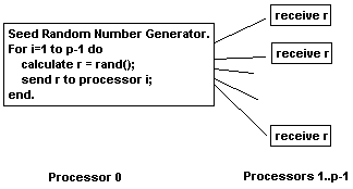 |
| Figure 5 Random number de-synchronization |
At the end of the computation we must send the partial estimates computed on each processor back to processor 0, which will then use those estimates to compute the final estimate. Since the only statistics that need to be communicated are the number of accepted points and the number of rejected points, we can communicate the information using a call to MPI_Reduceall with MPI_SUM used as the operation (figure 6).
/*compute the result*/ sum = (float)accept/(float)count * bounding_volume; MPI_Allreduce(&sum, &global_sum, 1, MPI_DOUBLE, MPI_SUM, MPI_COMM_WORLD); global_sum /= nproc; |
Using the algorithms and parallelization described above, a high-dimensional integral estimator was written in C using MPI. Results were collected using the BYU open lab machines, a collection of Hewlett Packard 9000 workstations with processor speeds ranging from 80 to 180 MHz connected over a 10 Mbps shared Ethernet line. During collection of the data, each run of the algorithm was repeated five times and the results were averaged. This was done to help offset the high variance in execution time that the machines in the open labs often exhibit.
Speedup was calculated by running the algorithm on 1, 2, 4, 8, and 16 processors with 100,000,000 generated points. The results are shown in Figure 7 and Table 1. Because the communication structure is minimal, we would expect that the measured speedup is close to the ideal speedup. For small numbers of processors, this is actually the case. Starting at 8 processors, though, the measured speedup falls significantly below the ideal speedup. This phenomenon is attributed to the architecture of the parallel system. For 8 processors or more, communication between processors now involves crossing at least one hub. Note, however, that the measured slope from 8 processors to 16 processors is close to the ideal slope for the same number of processors, implying that with the limits of the architecture taken into account (i.e., crossing hubs), the measured speedup actually does follow the ideal speedup.
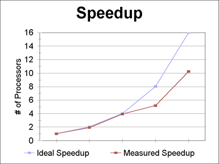 |
| Figure 7
Ideal vs. measured speedup using integral 1 with 100,000,000 generated points. |
| # Processors | Speedup |
| 1 | 1.00 |
| 2 | 1.92 |
| 4 | 3.92 |
| 8 | 5.16 |
| 16 | 10.24 |
To test this assertion, another set of tests was run and program execution time was collected for sample sizes ranging from 10,000 points to 10,000,000 points using 10 processors. The results of this graph, shown in figure 8 support the claim. As the number of samples increased by a factor of 10, the execution time increased by the same factor (hence the "linear" curve). Since this data was collected with a 10-processor system, the hub-crossing delays are included, implying that no additional overhead is incurred as the problem scales.
Figures 7 and 8 give a general indication that parallel Monte Carlo techniques are quite scalable. This is further supported by the communication structure. Communication bottlenecks can occur only at the beginning and at the end of the computation, since communication is performed nowhere else. And even at these points, efficient algorithms do exist for random number generator de-synchronization and all-to-all broadcasts, so that with careful algorithm selection these potential bottlenecks can be avoided. The result is an algorithm that scales extremely well with both problem size and processor count.
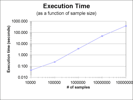 |
| Figure 8 Parallel execution time as a function of sample size |
To ease the task of preparing integrals for estimation, a simple script format was designed and implemented that allows integrals to be specified via an input file at runtime. Without this, the code would have to be modified for each integral, with varying amounts of changes needed for each integral depending on its dimension. Each function, whether it specifies an interval or the integrand itself, is parsed into an internal representation suitable for run-time evaluation [Hel].
All of the results listed in section 6.1 used this interpreted model. Since it is interpreted, it is slower than compiled code. Figure 9 shows the serial execution time of integral 1 from section 1 using interpreted functions verses the serial execution time of integral 1 with the functions hardcoded into the program. The test was also performed on integral 2. Although a graph is not shown, the results are similar. Table 2 shows the results of the tabulated data for both integrals 1 and 2. The data suggests that interpreted functions increase the computation time by about one-third. Whether or not the added expense incurred by interpreted functions is warranted depends almost entirely upon the application. Figure 10 shows the scripted version of integral 1.
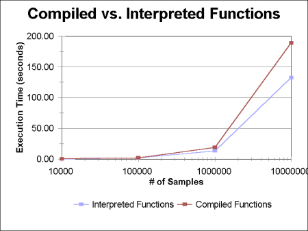 |
| Figure 9 Execution time of compiled functions vs. Interpreted functions. |
| Integral 1 | Integral 2 | |||
| Iterations | Compiled | Interpreted | Compiled | Interpreted |
| 10000 | 0.1336 | 0.191 | 0.1178 | 0.1544 |
| 100000 | 1.328 | 1.8912 | 0.9906 | 1.5328 |
| 1000000 | 13.2694 | 18.8954 | 9.8876 | 15.3146 |
| 10000000 | 132.7122 | 188.9535 | 98.87 | 153.2284 |
#This is the script defining integral in1 [variables] x y z [integrand] exp(x)*(y + 2*z) [intervals] x 0 2 y 0 "x" z 0 "x+y" [boundingbox] x 0 2 y 0 2 z 0 4 integrand 0 75 |
There is a lot of additional work that can be performed. For this project, the area-sampling method was used to obtained results. As the mean estimation technique is a superior method, an efficient means of parallelizing it would also be valuable. In addition, this system did not investigate the use of improper integrals - integrals with one or more intervals that extend to infinity. For this approach, the area-sampling method would require extensive modification, as it is impossible to get a non-infinite bounding box if an interval extends towards infinity.
The purpose of this project has been to investigate the feasibility of parallelizing Monte Carlo methods for estimating high-dimensional integrals. Because of the non-communicative nature of MC methods for estimating integrals, it was thought that they would parallelize well. We found this to be the case. The speedups that are obtainable seem restricted only by the limits of the underlying architecture. The value of these results are high. For the most part, automated tools such as Maple and Mathematica are capable of solving integrals up to four and five dimensions, but they generally do quite poorly beyond that [Whi]. Parallel Monte Carlo algorithms provide an efficient means for reaching beyond a five-dimensional limit; indeed, the speed with which they can return accurate results is limited only by the underlying architecture and number of available processors.
[Alu]    Aluru, Srinivas, G.M. Prahbu, and John Gustafson.  A Random Number
         Generator for Parallel Computers.  Parallel Computing,
         18(1992):839-847.

[Bur]    Burden, Richard L. and J. Douglas Faires. Numerical Analysis.
         PWS Publishing Co., Boston, 1993.

[Har]    Hartnock, Christoph.  Monte Carlo Integration.
         http://www-subatech.in2p3.fr/Sciences/Education/EMN/ch/mod/mcmeth/mcmeth.html,
	 November 1998.

[Hel]    Helfgott, Harald. Formulc: A Byte Compiler for Mathematical
         Functions.  http://www.cs.brandeis.edu/~hhelf/formulc/formulc.html,
	 November 1998.

[Shr]	 Shreider, Yu A. Method of Statistical Testing.  Elsevier,
         Amsterdam, 1964.

[Sob]	 Sobol', Ilia M. A Primer for the Monte Carlo Method.  CRC Press,
         Boca Raton, Florida, 1994.

[Whi]	 Interview with Dr. David G. Whiting, Professor of Statistics at
         Brigham Young University, October 1998.
 and
and
 .
.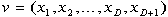 be a vector of D+1 random
values uniformly distributed within the bounding box.
be a vector of D+1 random
values uniformly distributed within the bounding box. for each dimension
 and
and
 then
then