Background
Expectation Maximization is a statistics algorithm used to estimate variance components for data in a mixed model. A mixed model can be thought of as a statistical experiment where the observations are taken from individuals that belong to different groups. The groups may belong to other groups, and so on. The difficulty comes in determining what effect those groups have on the variance between individuals. For example, taking measurements of patrons of different movie chains in different states. Which reactions are affected by the chain, by the state, by both, neither, etc.
Expectation Maximization "assumes individual response may be modeled as the sum of an overall population effect, a random individual deviation, and random errors. When individuals are nested within families or companies, this source or variability should also be considered."
The Expectation maximization process is roughly this. Assume we know some variance components correctly - the variance of the individuals without influence by other factors. Calculate the other effects, pretending those values were correct. After that calculation was correct, make the opposite assumption. Pretend the newly calculated values are correct and use them to calculate the original variance components. This is generally a stable process, and after some number of iterations, the calculated values can be said to be within an error epsilon of the expected value.
One problem statisticians face is that large data sets take a very long time to compute, as well as taking up a very large amount of space. By parallelizing the EM algorithm, not only can we decrease the time it takes to estimate these parameters, we can actually compute solutions to larger problems by taking advantage of extra storage on many machines.
Dr. Gilbert W. Fellingham of the Brigham Young University Statistics Department provided a serial implementation of an Expectation Maximization algorithm used to solve two-level mixed-effects models. The parallel implementation discussed by this paper evolved from this original implementation, and inherits any benefits or problems inherent in the original code. This paper outlines where those changes were made, and what effect those changes had on program performance.
PCAM - Analyzing the problem
The first step was to make serial optimizations to the code. The implementation provided by Dr. Fellingham only accessed the resources of one machine, and was forced to store much of its temporary data on disk because of space constraints. A parallel implementation would be able to use the memory of many machines, so the first order of business was to store all the matrixes in memory, rather than on the disk. By just removing disk access from the computation, the new code finished a small problem 4 times faster. (A small problem, so that it would fit on one machine).
Partitioning
The next step was to analyze the code to split it into parallel tasks. Using data decomposition, the matrixes of observations of individuals could be considered a single task. It is not economical to split up the four observation matrixes since they are often used together in the same equation. Using functional decomposition, the 20 different equations could be considered separate tasks as well. Due to data replication and data dependency considerations, the functional decomposition is not particularly effective for achieving speedup, but the analysis helps in determining the communication requirements.
Communication
After careful analysis of the dependencies between the equations, and some fancy mathematical rewriting done by Dr. Worth, only two points of communication are required during each iteration - when group values are computed from the individual matrixes. The first is used to distribute the temporary matrices used in passes 3 and 4. The second communication gathers the variances of all the individuals to compute the change between iterations (to determine if its time to stop.)
Agglomeration
The statistical equations can be split into 6 groups, each group dependant upon the previous for data. So calculation of various equations cannot be split up into different tasks because the second group can't start until the first finished, the third can't start until the second finishes, etc. (Future work could look into striping the W, X, y and Z matrixes and pipelining the computation. I doubt this would work though.)
Mapping
Because the individual matrixes were small in size, it was not necessary to split them across machines. A much simpler and faster implementation distributed the matrixes for different individuals across many machines using a __________ approach. This was more complicated than an MPI_Scatter call because the matrixes were not a uniform size, and the rows and columns of each matrix had to be kept together to reduce communication costs. While splitting the matrixes along group boundaries sounds attractive, it is less effective. Since groups are not constrained to be any particular size, this leads to poor load balancing, while providing no advantages in communication.
One Last Optimization
Because there are actually 5 different arrays of matrixes holding temporary results, there would need to be 5 communications at each of the communication points instead of 1. The parallel implementation has one more optimization allowing the data sections of the matrixes to be allocated contiguously for all 5 arrays. This removes 8 log2 n network latencies from the Allreduce sections.
The Parallel Code
The actual implementation splits up the computation into six stages (making the theoretic model easier to compute) with two communication points. Here is a top level view of the code:
Redundant computation is performed during steps 2,3 and 6 during which matrixes related to group value are computed for use in the following passes (3,4 and 1 respectively). As more processes are added, the redundant computation takes a larger percent of time. The following model gives rough theoretic values for computation times for each pass.
|
|
|
| pass1 | f1(pa, pb, pc) * N/p |
| Allreduce | 2 log2 [5m* f2(pa, pb, pc)] |
| pass2 | f3(pa, pb, pc) * m |
| pass3 | f4(pa, pb, pc) * m |
| pass4 | f5(pa, pb, pc) * N/p |
| pass5 | f6(pa, pb, pc) * N/p |
| Allreduce | 2 log2 [5+2m* f2(pa, pb, pc)] |
| pass6 | f4(pa, pb, pc) * m |
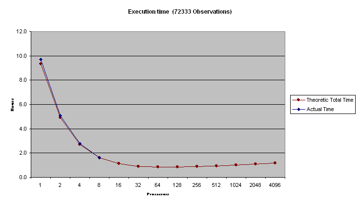
The PEM program was executed on 1, 2, 4 and 8 233 MHz Pentium Pro processors. The algorithm was tested on small and moderately sized data sets. The speed-up results are as follows
Costs for the scatter and gather are given below.
Scatter:
Table 1 - Scatter
| parameters | log2 p * ( latency + 24 bytes / bandwidth ) |
| individuals | log2 p * ( latency + m*4 bytes / bandwidth) |
| observations | log2 p * ( latency + K*4 bytes / bandwidth) |
| matrixes | ((p-1)* latency) + 8N * (pa+pb+pc+1) bytes / bandwidth |
| matrixes | ((p-1)*latency) + pb * 8 bytes / bandwidth |
We ran the code on 233MHz Dual Pentium machines on 100Mbit Ethernet using an MPI implementation for NT written by David Ashton. Actual Results are four 1, 2, 4 and 8 processors.
Table 3 - 41915 individuals , 72333 observations
| # of processors |
|
|
|
| 1 |
|
|
|
| 2 |
|
|
|
| 4 |
|
|
|
| 8 |
|
|
|
Table 4 - 143 individuals, 777 observations
| # of processors | Time per iteration | Total Time | speed-up |
| 1 | |||
| 2 | |||
| 4 | |||
| 8 | .075 | 43 seconds |

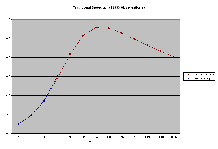
Figure 1
No actual results are available for scaled speedup; however, the model suggest behavior as shown below.
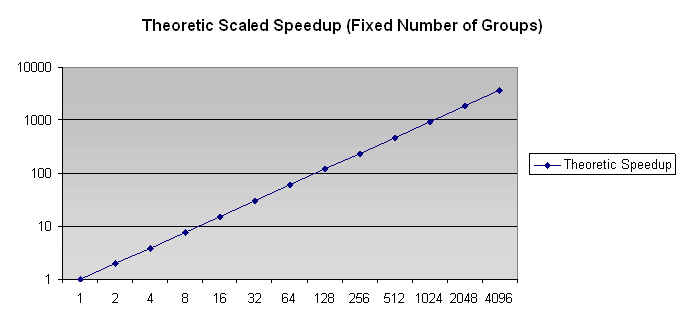
Figure 2
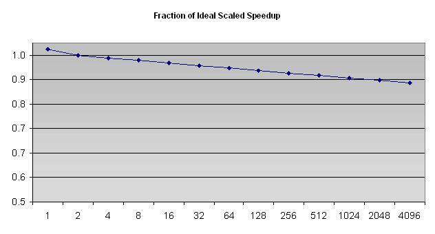
The most important result of all this work, though, is not the speedup.
By parallelizing the Expectation Maximization algorithm problems that were
intractable before are now computable. The BYU statistics department provided
three data sets, the first two they have solutions (or at least tentative
solutions) to. The third data set they cannot solve, but the Parallel Expectation
Maximization method did just fine.
Here is an Excel Spreadsheet to determine space
complexity of this code